Physics 238—Intermediate Physics Lab
Homework Assignment #3
Due Friday, March 14, 2025, 1:15 p.m.
In the torsional oscillator experiment, you found that the linear damping model did not describe the trial with air drag very well. In this assignment, you will see how to use Mathematica to numerically integrate the equations of motion, and then use that model to fit your data with air drag.
This work is presented here as a sequence of assignments. If you find it convenient, you may simply turn in one Mathematica notebook with your results, but please trim out irrelevant material before printing and submitting it.
This assignment is fairly long; it will be weighted as two homework assignments.
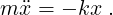
Consider a mass m attached to an ideal horizontal spring with spring constant k. The differential equation governing the motion is then simply
| (1) |
Take the initial conditions to be x(0) = x0 and ẋ(0) = v0. Your goal is to follow the evolution of the system with time, for times running from 0 to 10 seconds.
To be concrete, take the following numerical values:
| Variable | Value | Units | Description |
| k | 1.5 | N/m | Spring constant |
| m | 0.08 | kg | Mass, 80 g. |
| x0 | 0.80 | m | Initial position |
| v0 | 0.0 | m/s | Initial velocity |
| tstop | 10 | s | Total time to run |
Start Mathematica. Put a title at the top of your notebook. (Use the Format → Style menu. “Title” is rather large; feel free to pick something smaller.)
Put your name in a text cell near the top. Also give the date. (The command DateString[] is handy for this.) I also find it convenient to start each notebook with Clear["Global‘*"] to erase any possible lingering definitions from earlier work.
Add in the physical constants:
    k = 1.5 (* Spring constant *);
    m = 0.08 (* mass *);
You can add an in-line comment in Mathematica by enclosing text in (* and *). This is a helpful way to document your variables. Note too the trailing semicolon—it keeps Mathematica from printing out the result of each line.
It is also handy to add in a definition for the expected angular frequency and period,
| ω | =  | ||
| T | =  . . |
(You can enter the square root either by using the Classroom Palette or by typing Sqrt[k/m]. You can enter π by typing Pi, by using the Classroom Palette, or by the keyboard shortcut Escape p Escape.)
Although it is possible to solve Eq. 1 analytically, that won’t always be the case. Fortunately, it is also possible to approximate the solution numerically.
Mathematica has a built-in function, NDSolveValue, that handles numerical integration very efficiently. It chooses the numerical method and optimal step size automatically, and simply returns a function that you can evaluate to find the result. You can use it as follows:
    x0 = 0.8 (* Initial position *);
    v0 = 0 (* Initial velocity *);
    tstop = 10 (* Total time to run *);
    shm = NDSolveValue[
        {m x’’[t] == -k x[t], x[0] == x0, x’[0] == v0},
         x,
        {t, 0, tstop}
    ]
The NDSolveValue function takes three arguments, separated by commas and enclosed in square brackets. Since the arguments are fairly long, this example breaks them across several lines—one line for each argument. The first argument (in curly braces) is the list of equations to solve, including any boundary conditions. Note that in Mathematica, x’[t] means to take a derivative of x[t]. Note too that the equations are written with a double equals sign.1 The second argument tells NDSolveValue what to solve for, and the third tells it the independent variable (t) and over what time interval to run the integration. The answer is returned as a function (shm[t]) that can be evaluated and plotted.
Copy and Paste Warning:
You are encouraged to copy and paste code from this document, but you might have to
manually make some small edits. For example, the derivatives in x’[t] and x’’[t] are made
with the single quote key on the keyboard, but some software may render them as “smart
quotes” instead. If you get a syntax error, try deleting the quote marks and re-typing them in by
hand.
Please give each assignment an appropriate header in your notebook (e.g. by selecting a reasonable entry from the Format → Style menu). Please make sure all graphs have appropriate labels. Any comments may be inserted using text cells.
Assignment 1: Plot the result for x(t) for t = 0 to 10 s. You can do that with a simple command such as
Plot[shm[t], {t, 0, tstop}]
You should get a cosine function that oscillates between 0.8 and -0.8.
This simple plot is fine for trying things out, but when you are preparing a plot for presentation or submission, you should make sure the axes are labeled, and that each plot either has a label or is described by an appropriate caption in your final document. Most graphs also include a frame around the whole plot. The default font used by Mathematica for the axis labels is also quite small, and is often hard to read. Finally, it is often helpful to make the plot larger; this example makes it 70% of the page width.
    Plot[shm[t], {t, 0, tstop},
        PlotLabel -> "Simple Harmonic Motion",
        LabelStyle -> Larger, Frame -> True,
        FrameLabel -> {"t (s)", "x (m)"}, ImageSize -> Scaled[0.7]]
In the interest of saving space, examples in this writeup will not show these options every time, but you should include them as needed before submitting your final noteboook.
Assignment 2: In this problem, you can also compute the motion analytically,
Compute the analytic prediction for x(10) and compare to Mathematica’s value shm[10]. Do
they agree? If not, how much do they differ by?
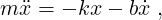
Next, you will consider what happens if you add a linear damping term, also known as viscous damping. Specifically, consider the new equation
| (2) |
where b is the damping coefficient.
Assignment 3: Set b = 0.1Ns∕m and solve Eq. 2 for the resulting motion. Call your answer
damped[t]. Plot the result for x(t) for t = 0 to 10 s. Note that Mathematica tries to zoom
in on the “interesting” part of the graph. You should force Mathematica to show
the full range by adding the option PlotRange->All. Also add in appropriate axis
labels.
Finally, you will consider a different model for damping, namely quadratic damping. This would be appropriate for resistance due to air drag, for example.
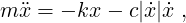
Specifically, consider the new equation
| (3) |
where c is a constant. (The combination -|ẋ|ẋ has the magnitude of v2, but always has a sign opposite v, so that the drag force opposes the motion.) In Mathematica, you can take the absolute value with the Abs[ ] function.
Assignment 4: Set c = 0.1Ns2∕m2 and solve Eq. 3 for the resulting motion. Call your answer airdrag[t]. Plot airdrag[t] vs. t for t = 0 to 10 s. On the same graph, include the result for viscous drag from the previous part. One way to plot two functions at once is by giving the Plot command a list of functions (enclosed in curly braces) instead of just a single function:
    Plot[{damped[t], airdrag[t]}, {t, 0, tstop},
          PlotLegends -> {"Viscous damping", "Air drag"}]
When you have more than one plot, it is important to label them. The PlotLegends option does that. It takes a list of plot labels (enclosed in curly braces)—one label for each plot. As always, add in appropriate readable labels.
Assignment 5: Comment on the qualitative differences between linear and quadratic damping. Do they correspond to what you observed in the torsional oscillator experiment?
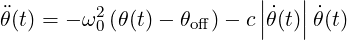
Lastly, you will use Mathematica to fit Eq. 3 to your data from the torsional oscillator experiment where the drag was provided by the air paddles. Specifically, assume that the differential equation is
| (4) |
subject to the initial conditions θ(0) = θ0 and  (0) = v0. (The constant θoff accounts for the fact
that the voltage was not exactly zero when the oscillator was at equilibrium.)
(0) = v0. (The constant θoff accounts for the fact
that the voltage was not exactly zero when the oscillator was at equilibrium.)
You will use NonlinearModelFit to fit Eq. 4 to your data. There are actually 5 fit parameters: 3 for the differential equation: ω0, θoff, c, and two for the initial conditions: θ0 and v0.
Roughly speaking, the plan is to use NonlinearModelFit to apply the principle of least squares. That is, you will pick a particular set of parameters, and Mathematica will use NDSolveValue to create a model solution, and evaluate χ2 for that model. Then Mathematica will try varying one (or more) of the parameters slightly to see if χ2 increases or decreases, and continue varying parameters until a minimum is found.
You have already seen how NonlinearModelFit sometimes needs help finding sensible starting guesses for this process. A second challenge in this problem is that Mathematica will tend to keep calling NDSolveValue over and over again with the same parameters to calculate χ2 such that the process becomes unreasonably slow. Fortunately, there is a variant function called ParametricNDSolveValue that avoids this problem by temporarily storing (or “caching”) computed solutions. (This use of ParametricNDSolveValue is suggested in the NonlinearModelFit help page. See the first example under “Generalizations & Extensions”.)
To get started, perform the following steps:
         dataPlot = ListPlot[data, PlotStyle -> Red, PlotRange -> All,
                     LabelStyle -> Larger,
                     AxesLabel -> {"t (s)", "Angle (radians)"},
                     ImageSize -> Scaled[0.8]];
You do not need to print the plot just yet.
     Clear[\[Omega]0, c, \[Theta]0, v0, \[Theta]off]
     airdrag =
      ParametricNDSolveValue[
         { \[Theta]’’[t] == - \[Omega]0^2 ( \[Theta][t] - \[Theta]off ) -
                              c Abs[\[Theta]’[t]] \[Theta]’[t],
           \[Theta][0] == \[Theta]0, \[Theta]’[0] == v0
         },
         \[Theta],
        {t, 0, 30}, {\[Omega]0, c, \[Theta]0, v0, \[Theta]off}]
The first line ensures that any earlier definitions of the parameters from previous assignments are cleared. Note that you can enter θ directly; the form shown here is the plain text input form. If you copy and paste this code, Mathematica ought to insert the θ for you. Note too that many PDF renderers will change the single quote marks to “Smart” quotes, and you may have to manually change them back to single quote marks.
Plot[airdrag[2.5, 0.5, 0.7, -0.02, 0.1][t], {t, 0, 30}]
Assignment 6: It is important to start with reasonable guesses for all the parameters. The Manipulate function is handy for this. Try the following command:
Manipulate[
    Show[{
        dataPlot,
        Plot[airdrag[\[Omega]0, c, \[Theta]0, v0, 0][t], {t, 0, 30},
            PlotRange -> All]
    }],
    {{\[Omega]0, 2.5}, 2.0, 3.0, 0.01, Appearance -> "Labeled"},
    {{c, 0.5}, 0.1, 2.0, 0.05, Appearance -> "Labeled"},
    {{\[Theta]0, 0.5}, -1, 1, 0.05, Appearance -> "Labeled"},
    {{v0, 0}, -4, 4, 0.05, Appearance -> "Labeled"}
 ]
This command will produce a plot showing the data (which you made earlier) and the airdrag model, along with sliders allowing you to control 4 parameters: ω0, c, θ0, and v0. (For simplicity, this plot sets θoff = 0. You may adjust that manually if needed.) Each slider is controlled by a list (inside curly braces) of settings. For example,
{{c, 0.5}, 0.1, 2.0, 0.05, Appearance -> "Labeled"}
will give the c parameter an initial value of 0.5, and vary it between 0.1 and 2.0 in steps of 0.05. The Appearance -> "Labeled" command means the value for the parameter will appear as a label to the right of the slider. A small + sign next to the slider opens up additional controls.
Adjust the sliders to get a reasonable first guess at a fit. Adjust the ranges in the Manipulate command if you need to. List your parameters here.
Assignment 7: Now that you have a reasonable first guess at the fit parameters, you can use them to run NonlinearModelFit. The syntax is similar to what you have used before, but it is important to remember that the model gets input as
airdrag[\[Omega]0, c, \[Theta]0, v0, \[Theta]off][t]
You will probably see some warning messages, but if Mathematica is successful, you will get a FittedModel output. Test your result with a plot:
Show[{dataPlot, Plot[airdragFit[t], {t, 0, 30}, PlotRange -> All]}]
Adjust your initial guesses until you are satisfied with the fit. Include the graph with the fit overlaying the data in your final submission.
Assignment 8: List the fit parameters, along with their uncertainties. (The
"ParameterConfidenceIntervalTable" is appropriate here.) Again, you may see some warning
messages, but if the fit looks good you may ignore them.
Assignment 9: Find the root mean square error (RMSE) for the fit. Note that the units are radians. Is your value reasonable for the fit? Do you note any significant systematic errors?
Assignment 10: Consider the correlation between the different parameters. A useful way to display this is with MatrixForm[airdragFit["CorrelationMatrix"]]. Are there any large correlations? (You may ignore any correlation with an absolute value less than 0.5.) Qualitatively, can you relate any of those correlations to your observations varying the sliders? For example, if the values for ω0 and c display a negative correlation, than increases in ω0 can be at least somewhat offset by decreasing c. Such a correlation would show up as the 1st row, 2nd column.